boilercv

Computer vision routines suitable for nucleate pool boiling bubble analysis.

Example

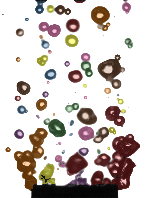
Overlay of the external contours detected in one frame of a high-speed video. Represents output from the “fill” step of the data process.

Fig. 1 Vapor bubbles with false-color overlay to distinguish detected contours. Contours tend to represent single bubbles or groups of overlapping bubbles.

Overview

The data process graph shows the data process, and allows for individual steps in the process to be defined indpendently as Python scripts, Jupyter notebooks, or even in other languages like Matlab. The process is defined in dvc.yaml as as series of “stages”. Each stage has dependencies and outputs. This structure allows the data process graph to be constructed, directly from the dvc.yaml file. This separates the concerns of data management, process development, and pipeline orchestration. This project reflects the application of data science best practices to modern engineering wokflows.

Try it out inside this documentation

If you see a “Run code” button like the one below, you can modify and re-run the code on the page. In any page with collapsed code sources and a “Run code button” you can do the following:

• Click “Run code”

• Wait until the dialog says “ready”

• Expand the first code cell on that page by clicking “Show code cell source,”

• Click “restart & run all”

You will see code cell output in the expanded input cells, and can compare it to the static output beneath it. You may also tweak values in the code and re-run it to get different outputs! Try running code below, then modify the code (e.g. to 1 + 1) and run it again! Note that it may take awhile for the “ready” dialog to appear if nobody has run code in these docs for awhile.

You may also click the binder link at the top of this page to open a JupyterLab instance with runnable Jupyter notebooks, though keep in mind that some notebooks exceed the resources allotted to the binder instance.

Run code

print("hello world!")

Usage

If you would like to adopt this approach to processing your own data, you may clone this repository and begin swapping logic for your own, or use a similar architecture for your data processing. To run a working example with some actual data from this study, perform the following steps:

1. Clone this repository and open it in your terminal or IDE (e.g. git clone https://github.com/softboiler/boilercv.git boilercv).

2. Navigate to the clone directory in a terminal window (e.g. cd boilercv).

3. Create a Python 3.11 virtual environment (e.g. py -3.11 -m venv .venv on Windows w/ Python 3.11 installed from python.org).

4. Activate the virtual environment (e.g. .venv/scripts/activate on Windows).

5. Run pip install requirements/requirements.txt to install boilercv and other requirements in an editable fashion.

6. Delete the top-level data directory, then copy the cloud folder inside tests/data to the root directory. Rename it to data.

7. Copy the data folder from tests/root to the root of the repo.

8. Run dvc repro to execute the data process up to that stage.

The data process should run the following stages: preview_binarized, preview_gray, find_contours, fill, and preview_filled. You may inspect the actual code that runs during these stages in pipeline/boilercv_pipeline/stages, e.g. find_contours.py contains the logic for the find_contours stage. This example happens to use Python scripts, but you could define a stage in dvc.yaml that instead runs Matlab scripts, or any arbitrary action. This approach allows for the data process to be reliably reproduced over time, and for the process to be easily modified and extended in a collaborative effort.

There are other details of this process, such as the hosting of data in the data folder in a Google Cloud Bucket (alternatively it can be hosted on Google Drive), and more. This has to do with the need to store data (especially large datasets) outside of the repository, and access it in an authenticated fashion.

Data process graph

This data process graph is derived from the code itself. It is automatically generated by dvc. This self-documenting process improves reproducibility and reduces documentation overhead. Nodes currently being implemented are highlighted.

flowchart TD node1["binarize"] node2["convert"] node3["data\models\modelfun-3.11.dillpickle.dvc"] node4["data\models\modelfun-3.12.dillpickle.dvc"] node5["data\thermal.dvc"] node6["fill"] node7["find_contours"] node8["find_objects"] node9["find_tracks"] node10["get_thermal_data"] node11["preview_binarized"] node12["preview_filled"] node13["preview_gray"] node14["skip_cloud"] node1-->node6 node1-->node7 node1-->node11 node1-->node12 node2-->node1 node2-->node13 node3-->node10 node4-->node10 node5-->node10 node6-->node8 node6-->node9 node6-->node12 node7-->node6 node7-->node8 node8-->node9 node10-->node9 node14-->node2 node15["data\examples.dvc"] node16["data\notebooks.dvc"] node17["data\samples.dvc"]