Find objects#
Find bubble size using two different approaches.
Show code cell source
from collections.abc import Iterable

from boilercv_dev.docs.nbs import get_mode, init
from boilercv_pipeline.dfs import limit_group_size
from boilercv_pipeline.models.column import Col, convert, rename
from boilercv_pipeline.models.deps import get_slices
from boilercv_pipeline.models.df import GBC, agg
from boilercv_pipeline.models.subcool import const
from boilercv_pipeline.sets import get_contours_df2, load_video
from boilercv_pipeline.stages.find_objects import FindObjects as Params
from boilercv_pipeline.stages.find_tracks import convert_col
from boilercv_pipeline.units import U
from devtools import pprint
from geopandas import GeoDataFrame, points_from_xy
from matplotlib.pyplot import subplots
from more_itertools import one, only
from numpy import pi, sqrt
from pandas import DataFrame, IndexSlice, NamedAgg, concat
from seaborn import scatterplot
from shapely import LinearRing, Polygon

from boilercv.data import FRAME
from boilercv.images import scale_bool

PARAMS = None
"""Notebook stage parameters."""
MODE = get_mode()
"""Notebook execution mode."""
Params.hide()
Show code cell source
if isinstance(PARAMS, str):  # pyright: ignore[reportUnnecessaryIsInstance]
    params = Params.model_validate_json(PARAMS)
elif MODE == "docs":
    preview_frame_count = 10
    params = Params(
        context=init(mode=MODE),
        compare_with_trackpy=True,
        include_patterns=const.nb_include_patterns,
        slicer_patterns=const.nb_slicer_patterns,
    )
else:
    params = Params(context=init(mode=MODE), only_sample=True)
params.set_display_options()
data = params.data
dfs = only(params.dfs)
C = params.cols

slices = get_slices(one(params.filled_slicers))
frames_slice = slices.get(FRAME, slice(None))
contours = get_contours_df2(one(params.contours)).loc[IndexSlice[frames_slice, :], :]
frames = contours.reset_index()[FRAME].unique()
preview_frame_count = round(0.619233215798799 * len(frames) ** 0.447632153789354)

# # ? Produce reduced-size docs data
# from pathlib import Path
# from boilercv_pipeline.sets import save_video
# save_video(
#     load_video(one(params.filled), slices={FRAME: range(500)}),
#     Path("docs/data/filled/2024-07-18T17-44-35.nc"),
# )
# contours.loc[frames, :].to_hdf(
#     "docs/data/contours/2024-07-18T17-44-35.h5",
#     key="contours",
#     complib="zlib",
#     complevel=9,
# )

M_PER_PX = U.convert(3 / 8, "in", "m") / (202 - 96)
U.define(f"px = {M_PER_PX} m")

PALETTE = {C.approach_tp.val: "red", C.approach.val: "blue"}


def preview(
    df: DataFrame, cols: Iterable[Col] | None = None, index: Col | None = None
) -> DataFrame:
    """Preview a dataframe in the notebook."""
    params.preview(
        cols=cols,
        df=df,
        index=index,
        f=lambda df: df.groupby(C.frame(), **GBC).head(3).head(6),
    )
    return df


pprint(params)
Show code cell output
FindObjects(
    context={
        'boilercv_pipeline': BoilercvPipelineContext(
            roots=Roots(
                data=PosixPath('/home/runner/work/boilercv/boilercv/docs/data'),
                docs=PosixPath('/home/runner/work/boilercv/boilercv/docs'),
            ),
            kinds={},
            track_kinds=False,
        ),
    },
    deps=Deps(
        context={
            'boilercv_pipeline': BoilercvPipelineContext(
                roots=Roots(
                    data=PosixPath('/home/runner/work/boilercv/boilercv/docs/data'),
                    docs=PosixPath('/home/runner/work/boilercv/boilercv/docs'),
                ),
                kinds={},
                track_kinds=False,
            ),
        },
        stage=PosixPath('/home/runner/work/boilercv/boilercv/packages/pipeline/boilercv_pipeline/stages/find_objects'),
        nb=PosixPath('/home/runner/work/boilercv/boilercv/docs/notebooks/find_objects.ipynb'),
        filled=PosixPath('/home/runner/work/boilercv/boilercv/docs/data/filled'),
        contours=PosixPath('/home/runner/work/boilercv/boilercv/docs/data/contours'),
    ),
    outs=Outs(
        context={
            'boilercv_pipeline': BoilercvPipelineContext(
                roots=Roots(
                    data=PosixPath('/home/runner/work/boilercv/boilercv/docs/data'),
                    docs=PosixPath('/home/runner/work/boilercv/boilercv/docs'),
                ),
                kinds={},
                track_kinds=False,
            ),
        },
        dfs=PosixPath('/home/runner/work/boilercv/boilercv/docs/data/e230920/objects'),
        plots=PosixPath('/home/runner/work/boilercv/boilercv/docs/data/e230920/objects_plots'),
    ),
    scale=1.3,
    marker_scale=20.0,
    precision=3,
    display_rows=12,
    data=Data(
        context={
            'boilercv_pipeline': BoilercvPipelineContext(
                roots=Roots(
                    data=PosixPath('/home/runner/work/boilercv/boilercv/docs/data'),
                    docs=PosixPath('/home/runner/work/boilercv/boilercv/docs'),
                ),
                kinds={},
                track_kinds=False,
            ),
        },
        dfs=Dfs(
            src=<DataFrame({
            })>,
            dst=<DataFrame({
            })>,
            trackpy=<DataFrame({
            })>,
            centroids=<DataFrame({
            })>,
            geo=<DataFrame({
            })>,
        ),
        plots=Plots(
            context={
                'boilercv_pipeline': BoilercvPipelineContext(
                    roots=Roots(
                        data=PosixPath('/home/runner/work/boilercv/boilercv/docs/data'),
                        docs=PosixPath('/home/runner/work/boilercv/boilercv/docs'),
                    ),
                    kinds={},
                    track_kinds=False,
                ),
            },
            composite=<Figure size 640x480 with 0 Axes>,
        ),
    ),
    sample='2024-07-18T17-44-35',
    only_sample=False,
    include_patterns=[
        '^.*2024-07-18T17-44-35.*$',
    ],
    frame_count=0,
    frame_step=1,
    slicer_patterns={
        '.+': {
            'frame': Slicer(
                start=None,
                stop=499,
                step=1,
            ),
        },
    },
    filled=[
        PosixPath('/home/runner/work/boilercv/boilercv/docs/data/filled/2024-07-18T17-44-35.nc'),
    ],
    filled_slicers=[
        {
            'frame': Slicer(
                start=None,
                stop=499,
                step=1,
            ),
        },
    ],
    times=[
        '2024-07-18T17-44-35',
    ],
    dfs=[
        PosixPath('/home/runner/work/boilercv/boilercv/docs/data/e230920/objects/objects_2024-07-18T17-44-35.h5'),
    ],
    cols=Cols(
        frame=LinkedCol(
            sym='Frame',
            unit='',
            sub='',
            raw='Frame',
            fmt='.0f',
            source=Col(
                sym='frame',
                unit='',
                sub='',
                raw='frame',
                fmt=None,
            ),
            latex='$\\mathsf{Frame}$',
        ),
        contour=LinkedCol(
            sym='Contour',
            unit='',
            sub='',
            raw='Contour',
            fmt='.0f',
            source=Col(
                sym='contour',
                unit='',
                sub='',
                raw='contour',
                fmt=None,
            ),
            latex='$\\mathsf{Contour}$',
        ),
        x=LinkedCol(
            sym='x',
            unit='px',
            sub='',
            raw='x (px)',
            fmt=None,
            source=Col(
                sym='xpx',
                unit='',
                sub='',
                raw='xpx',
                fmt=None,
            ),
            latex='$\\mathsf{x\\ \\left(px\\right)}$',
        ),
        y=LinkedCol(
            sym='y',
            unit='px',
            sub='',
            raw='y (px)',
            fmt=None,
            source=Col(
                sym='ypx',
                unit='',
                sub='',
                raw='ypx',
                fmt=None,
            ),
            latex='$\\mathsf{y\\ \\left(px\\right)}$',
        ),
        x_tp=LinkedCol(
            sym='x',
            unit='px',
            sub='',
            raw='x (px)',
            fmt=None,
            source=Col(
                sym='x',
                unit='',
                sub='',
                raw='x',
                fmt=None,
            ),
        ),
        y_tp=LinkedCol(
            sym='y',
            unit='px',
            sub='',
            raw='y (px)',
            fmt=None,
            source=Col(
                sym='y',
                unit='',
                sub='',
                raw='y',
                fmt=None,
            ),
        ),
        size=LinkedCol(
            sym='Size',
            unit='px',
            sub='',
            raw='Size (px)',
            fmt=None,
            source=Col(
                sym='size',
                unit='',
                sub='',
                raw='size',
                fmt=None,
            ),
            latex='$\\mathsf{Size\\ \\left(px\\right)}$',
        ),
        centroid=Col(
            sym='Centroid',
            unit='',
            sub='',
            raw='Centroid',
            fmt=None,
            latex='$\\mathsf{Centroid}$',
        ),
        geometry=Col(
            sym='Geometry',
            unit='',
            sub='',
            raw='Geometry',
            fmt=None,
        ),
        area=Col(
            sym='A',
            unit='px^2',
            sub='',
            raw='A (px^2)',
            fmt=None,
            latex='$\\mathsf{A\\ \\left(px^2\\right)}$',
        ),
        diameter=Col(
            sym='d',
            unit='px',
            sub='',
            raw='d (px)',
            fmt=None,
            latex='$\\mathsf{d\\ \\left(px\\right)}$',
        ),
        radius_of_gyration=Col(
            sym='r',
            unit='px',
            sub='',
            raw='r (px)',
            fmt=None,
            latex='$\\mathsf{r\\ \\left(px\\right)}$',
        ),
        approach_tp=ConstCol(
            sym='Approach',
            unit='',
            sub='',
            raw='Approach',
            fmt=None,
            val='Trackpy',
        ),
        approach=ConstCol(
            sym='Approach',
            unit='',
            sub='',
            raw='Approach',
            fmt=None,
            val='Centroids',
        ),
        sources=[
            LinkedCol(
                sym='Frame',
                unit='',
                sub='',
                raw='Frame',
                fmt='.0f',
                source=Col(
                    sym='frame',
                    unit='',
                    sub='',
                    raw='frame',
                    fmt=None,
                ),
                latex='$\\mathsf{Frame}$',
            ),
            LinkedCol(
                sym='Contour',
                unit='',
                sub='',
                raw='Contour',
                fmt='.0f',
                source=Col(
                    sym='contour',
                    unit='',
                    sub='',
                    raw='contour',
                    fmt=None,
                ),
                latex='$\\mathsf{Contour}$',
            ),
            LinkedCol(
                sym='x',
                unit='px',
                sub='',
                raw='x (px)',
                fmt=None,
                source=Col(
                    sym='xpx',
                    unit='',
                    sub='',
                    raw='xpx',
                    fmt=None,
                ),
                latex='$\\mathsf{x\\ \\left(px\\right)}$',
            ),
            LinkedCol(
                sym='y',
                unit='px',
                sub='',
                raw='y (px)',
                fmt=None,
                source=Col(
                    sym='ypx',
                    unit='',
                    sub='',
                    raw='ypx',
                    fmt=None,
                ),
                latex='$\\mathsf{y\\ \\left(px\\right)}$',
            ),
        ],
    ),
    compare_with_trackpy=True,
    guess_diameter=21,
    contours=[
        PosixPath('/home/runner/work/boilercv/boilercv/docs/data/contours/2024-07-18T17-44-35.h5'),
    ],
)
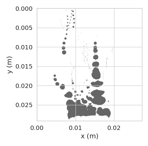
Data#
Load a video of filled contours and the contour loci and plot a composite of all frames to analyze.
Show code cell source
data.plots.composite, ax = subplots()
filled_path = one(params.filled)
with load_video(
    filled_path, slices={FRAME: frames[:: int(len(frames) // preview_frame_count)]}
) as video:
    filled_preview = scale_bool(video)
    composite_video = scale_bool(video).max(FRAME).values
    height, width = composite_video.shape[:2]
    ax.imshow(
        ~composite_video, alpha=0.6, extent=(0, width * M_PER_PX, height * M_PER_PX, 0)
    )
    preview_frames = filled_preview.coords[FRAME]
ax.set_xlabel(C.x().replace("px", "m"))
ax.set_ylabel(C.y().replace("px", "m"))


def preview_objects(df: DataFrame):
    """Preview objects."""
    return df.set_index(C.frame()).loc[preview_frames, :].reset_index()
Find size from filled contours using Trackpy#
Use Trackpy to find bubble size given the filled contours.
Show code cell source
if params.compare_with_trackpy:
    from trackpy import batch, quiet

    quiet()

    with load_video(filled_path, slices=slices) as video:
        filled = scale_bool(video)
        trackpy_cols = [*C.trackpy, C.x_tp, C.y_tp]
        data.dfs.trackpy = preview(
            cols=trackpy_cols,
            df=batch(
                frames=filled.values, diameter=params.guess_diameter, characterize=True
            )
            .pipe(C.frame.rename)
            .assign(**{
                C.frame(): lambda df: df[C.frame()].replace(
                    dict(enumerate(filled.frame.values))
                )
            })
            .pipe(rename, trackpy_cols)[[c() for c in trackpy_cols]],
        )
\(\mathsf{Frame}\) |
\(\mathsf{Size\ \left(px\right)}\) |
\(\mathsf{x\ \left(px\right)}\) |
\(\mathsf{y\ \left(px\right)}\) |
|---|---|---|---|
0 |
2.10 |
104. |
52.8 |
0 |
4.13 |
77.6 |
127. |
0 |
2.38 |
103. |
216. |
1 |
2.32 |
104. |
52.2 |
1 |
4.15 |
77.5 |
126. |
1 |
2.36 |
103. |
215. |
Find size from contours#
The prior approach throws out contour data, instead operating on filled contours. Instead, try using shapely to find size directly from contour data.
Prepare to find objects#
Prepare a dataframe with columns in a certain order, assign contour data to it, and demote the hiearchical indices to plain columns. Count the number of points in each contour and each frame, keeping only those which have enough points to describe a linear ring. Construct a GeoPandas geometry column and operate on it with Shapely to construct linear rings, returning centroids and the representative polygonal area. Also report the number of points in the loci of each contour per frame.
Show code cell source
data.dfs.centroids = preview(
    cols=C.centroids,
    df=contours.reset_index()
    .pipe(rename, C.sources)
    .pipe(limit_group_size, [C.frame(), C.contour()], 3)
    .assign(**{C.geometry(): lambda df: points_from_xy(df[C.x()], df[C.y()])})
    .groupby([C.frame(), C.contour()], **GBC)
    .pipe(
        agg,
        {
            C.centroid(): NamedAgg(C.geometry(), lambda df: LinearRing(df).centroid),
            C.area(): NamedAgg(C.geometry(), lambda df: Polygon(df).area),
        },
    ),
)
\(\mathsf{Frame}\) |
\(\mathsf{Contour}\) |
\(\mathsf{Centroid}\) |
|---|---|---|
0 |
0 |
POINT (158.84922695375144 302.15435718388176) |
0 |
1 |
POINT (196.5259972164771 301.30000101116354) |
0 |
2 |
POINT (115.76214846973382 303.32748111943545) |
1 |
0 |
POINT (158.98006982861273 302.285200058743) |
1 |
1 |
POINT (196.5259972164771 301.30000101116354) |
1 |
2 |
POINT (116.13783949626864 303.24042201831236) |
Split the centroid point objects into separate named columns that conform to the Trackpy convention. Report the centroids in each frame.
Show code cell source
data.dfs.geo = params.preview(
    cols=C.geo,
    df=data.dfs.centroids.assign(**{
        C.diameter(): lambda df: sqrt(4 * df[C.area()] / pi),
        C.radius_of_gyration(): lambda df: df[C.diameter()] / 4,
        C.size(): lambda df: df[C.radius_of_gyration()],
    }),
)
\(\mathsf{Frame}\) |
\(\mathsf{Contour}\) |
\(\mathsf{A\ \left(px^2\right)}\) |
\(\mathsf{d\ \left(px\right)}\) |
\(\mathsf{r\ \left(px\right)}\) |
|---|---|---|---|---|
0 |
0 |
220. |
16.8 |
4.19 |
0 |
1 |
396. |
22.5 |
5.62 |
0 |
2 |
944. |
34.7 |
8.66 |
0 |
3 |
69.0 |
9.37 |
2.34 |
0 |
4 |
837. |
32.6 |
8.16 |
Show code cell source
data.dfs.dst = preview(
    cols=C.dests,
    df=GeoDataFrame(data.dfs.geo).assign(**{
        C.x(): lambda df: df[C.centroid()].x,
        C.y(): lambda df: df[C.centroid()].y,
    })[[c() for c in C.dests]],
)
\(\mathsf{Frame}\) |
\(\mathsf{Contour}\) |
\(\mathsf{x\ \left(px\right)}\) |
\(\mathsf{y\ \left(px\right)}\) |
\(\mathsf{A\ \left(px^2\right)}\) |
\(\mathsf{d\ \left(px\right)}\) |
\(\mathsf{r\ \left(px\right)}\) |
|---|---|---|---|---|---|---|
0 |
0 |
159. |
302. |
220. |
16.8 |
4.19 |
0 |
1 |
197. |
301. |
396. |
22.5 |
5.62 |
0 |
2 |
116. |
303. |
944. |
34.7 |
8.66 |
1 |
0 |
159. |
302. |
218. |
16.7 |
4.17 |
1 |
1 |
197. |
301. |
396. |
22.5 |
5.62 |
1 |
2 |
116. |
303. |
949. |
34.8 |
8.69 |
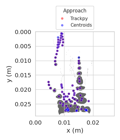
Compare approaches#
Compare Trackpy objects with contour objects. Here the guess radius for Trackpy object finding and contour perimeter filtering are matched to produce the same number of objects from each algorithm. Trackpy features more intelligent filtering, but takes much longer. Trackpy’s approach for finding local maxima in grayscale images is applied even to binarized images, exhaustively searching for high points in the binary image, adding to execution time.
The percent difference between the approaches is relatively low for this subset, suggesting the contour centroid approach is reasonable.
A warm color palette is used to plot Trackpy objects, and a cool color palette is used to plot contour centroids.
Show code cell source
trackpy_preview = (
    data.dfs.trackpy.pipe(preview_objects)[[C.y_tp(), C.x_tp()]].pipe(
        C.approach_tp.assign
    )
    if params.compare_with_trackpy
    else DataFrame()
)
centroids_preview = (
    data.dfs.dst.pipe(preview_objects)[[C.y(), C.x()]]
    .pipe(C.approach.assign)
    .pipe(convert, [convert_col(C.x, "m"), convert_col(C.y, "m")], U)
)
with params.display_options(scale=1.0):
    scatterplot(
        ax=ax,
        alpha=0.5,
        x=convert_col(C.x, "m")(),
        y=convert_col(C.y, "m")(),
        hue=C.approach(),
        palette=PALETTE,
        data=concat([trackpy_preview, centroids_preview]),
        legend=params.compare_with_trackpy,
    )
    if params.compare_with_trackpy:
        params.move_legend(ax, ncol=1)
data.plots.composite